How to use 3D models of the 2002-03-10 cold flare
1. Needed soft: IDL (8.0 or above)/SSW + GX_Simulator (preinstalled from SSW/packages: Solar software http://www.lmsal.com/solarsoft/).
2. Save all provided files in a local folder. This collection of files will let you to reproduce the results presented in http://adsabs.harvard.edu/abs/2016ApJ...822...71F
3. Launch GX_Simulator: IDL> GX
4. In the tab "Volume View" upload one of available models using
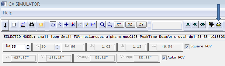
5. If more than one model has been imported into GX Simulator, make sure that the desired one has been selected on the right in the "model" tab:
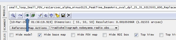
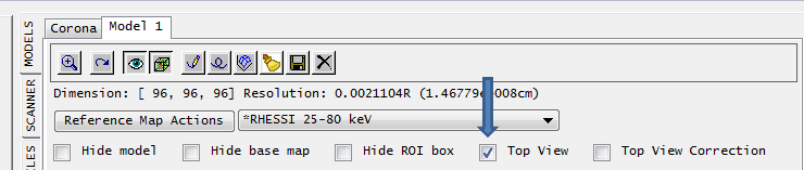
6. In the "Models" tab select "Top view":
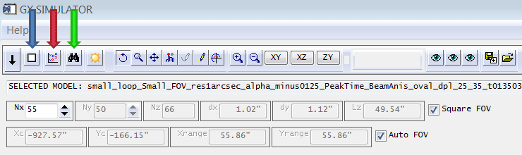
7. In the tab "Volume View" push button "Compute inscribing FOV" (blue arrow) and, once complete, "Zoom to FOV" (green arrow) and, finally, "COMPUTE RENDERING GRID" (red arrow):
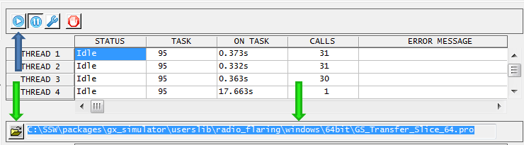
8. To compute MW (GS+FF) emission, select one of available fast codes (green arrows), e.g., "C:SSWpackagesgx_simulatoruserslibradio_flaringwindows64bitGS_Transfer_Slice_64.pro", in the "Scanner" tab and hit the button "Scan FOV" (blue arrow):
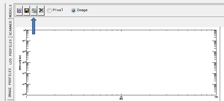
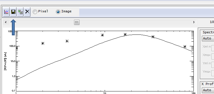
9. To make comparison between the computed and observed spectra in the "Image Profiles" tab, import provided *.ref file (for MW/NoRP data); make sure that the "Image" radio button is selected, which integrates emission over the image:
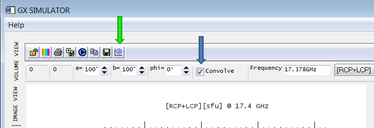
10. Now, in "image view," you may convolve the synthesized image (blue arrow) with a desired 2D Gaussian beam and then send the image (convolved or not) to Plotman for comparison with observed images (green arrow).
11. When emission has been computed, you can save the spectrum to a file (e.g., "Spectrum.sav") for further use outside the tool.
The spectrum can be retrieved in IDL:
- restore, 'Spectrum.sav'[,/relaxed_structure_assignment]
- freguency_gx=objxy->Get_XData()
- Flux_gx =objxy->Get_YData()
This can be compared with the original NoRP data file http://solar.nro.nao.ac.jp/norp/xdr/2002/03/norp20020310_0135.xdr
Note that changes of the volume rendering method in GX Simulator may result in noticeable changes in the computed spectrum if the original vertical grid step is too large. Future GS Simulator upgrades will allow changing this vertical step size for more precise computations.
12. Use the GX functionality to inspect the model and adjust it to fit emissions during other time frames.