How to use 3D models of the 2002-04-12 dense flare

1. Needed soft: IDL (8.0 or above)/SSW + GX_Simulator (preinstalled from SSW/packages: Solar software http://www.lmsal.com/solarsoft/).

2. Save all provided files in a local folder. This collection of files will let you to reproduce the results presented in http://adsabs.harvard.edu/abs/2016ApJ...816...62F

3. Launch GX_Simulator: IDL> GX

4. In the tab "Volume View" upload one of two available models using

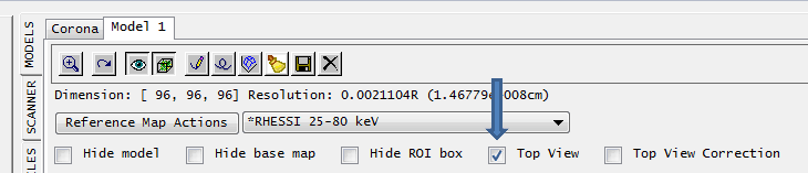
5. In the "Models" tab select "Top view"

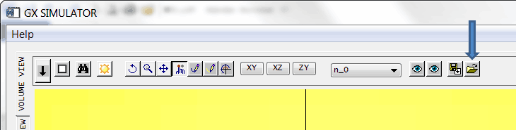
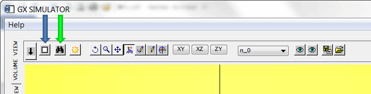
6. In the tab "Volume View" push button "Compute inscribing FOV" (blue arrow) and, once complete, "Zoom to FOV" (green arrow)

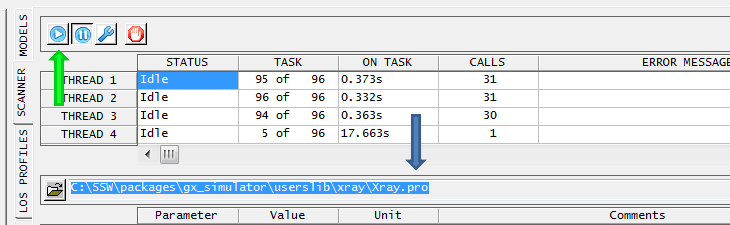
7. To compute X-ray emission, make sure that "C:\SSW\packages\gx_simulator\userslib\xray\Xray.pro" is selected in the "Scanner" tab and hit the button "Scan FOV"

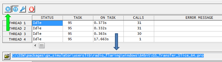
8. To compute MW (GS+FF) emission, select one of available fast codes, e.g., "C:\SSW\packages\gx_simulator\userslib\radio_flaring\windows\64bit\GS_Transfer_Slice_64.pro", in the "Scanner" tab and hit the button "Scan FOV"

9. To make comparison between the computed and observed spectra in the "Image Profiles" tab, import one of provided *.ref files (for either X-ray/RHESSI or MW/OVSA data)

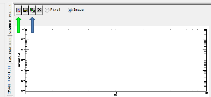
10. To make comparison between the computed and observed X-ray spectra in the "Plotman" tab on the left, (1) push the button "Send spectrum to Plotman" (green arrow above), and import one of provided *.xy files (for X-ray data) by the command file/overplot XY data from file.

11. Use the GX functionality to inspect the model and adjust it to fit emissions during other time frames.

Additional comments after GX upgrade on November, 2016

If you are using updated GX Simulator, some minor modifications of the use will be needed.

1. Given that an ability of scanning from an arbitrary view was added, after step 6 above, you have also "compute rendering grid":

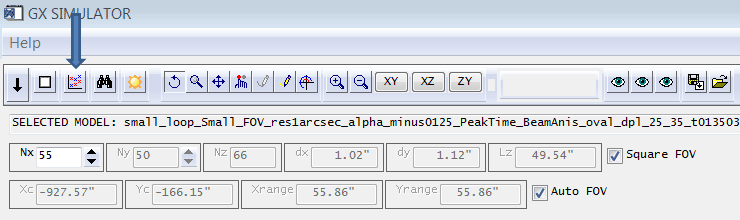
While doing so, you can also select the number of pixels in the image (here: Nx = 55, square FOV), which must not necessarily coincide with resolution of the model.

2. If more than one model has been imported into GX Simulator, make sure that the desired one has been selected on the right in the model tab:

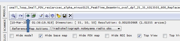
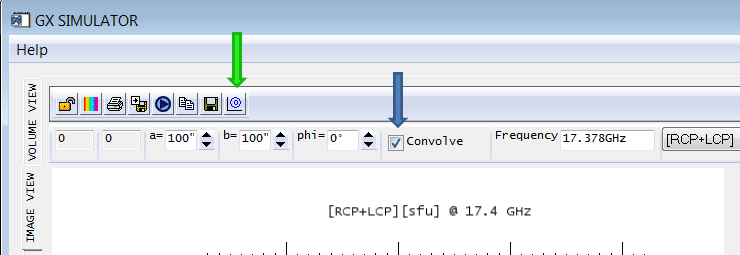
3. Now, in "image view", you may convolve the synthesized image (blue arrow) with a desired 2D Gaussian beam and then send the image (convolved or not) to Plotman for comparison with observed images (green arrow).