How to use 3D models of active regions
1. Needed soft: IDL (8.0 or above)/SSW + GX_Simulator (preinstalled from SSW/packages: Solar software www.lmsal.com/solarsoft/).
2. Save the chosen .GXM file in a local folder.
3. Launch GX_Simulator: IDL> gx_simulator [hit “Enter”]
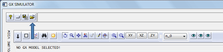
4. In the tab ‘Volume View’ upload the chosen model using Open button.
Push “OK”, if a warning about undefined variable appears. Push “No” when asked to proceed with the rendering grid computation. The file names contain the AR number, date, time, coordinates of the AR center, information about the chosen projection (top-view) and the magnetic field extrapolation code (NLFFF by A. Stupishin), and the model type. All models include the coronal part; the models with ‘chromo’ suffix contain also the chromospheric part.
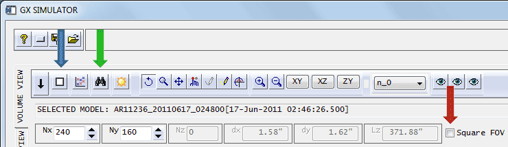
5. In the tab ‘Volume view’ uncheck the ‘Square FOV’ box (red arrow), then push ‘Compute inscribing FOV’ button (blue arrow) and then ‘Zoom to FOV’ button (green arrow).
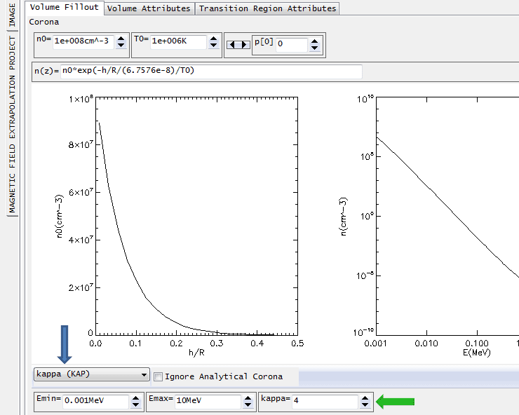
6. In the tab ‘Models → Volume Fillout’ select (blue arrow) the necessary plasma distribution type (‘free-free only’ for the model ignoring gyroresonance emission, ‘thermal’ for the Maxwellian distribution, or ‘kappa’ for the kappa-distribution). For the kappa distribution, you can also modify the kappa index (green arrow); hit “Enter” after modifying this parameter to make the changes into effect. Push “No” when asked to proceed with the rendering grid computation.
7. In the tab ‘Models → Volume Attributes’ check the ‘EUV: EBTEL DEM, Radio/Xray: stored n-T’ switch (blue arrow) (if not checked already), then modify as necessary the formulae describing the plasma heating (‘Q’ and ‘q0’ boxes) and various parameters of those formulae (‘q[0]’ – ‘q[4]’) (green arrows).
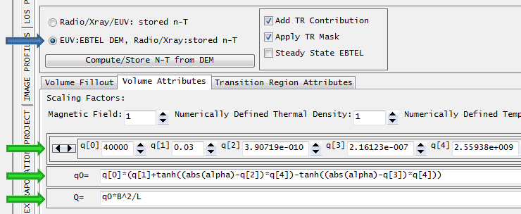
After modifying a parameter hit “Enter” to make the changes into effect. When asked to recompute n-T push “No” unless your changes are final, otherwise push “Yes” and wait until the computation is complete. Then, when asked to proceed with the rendering grid computation, push “Yes” and wait until the computation is complete.
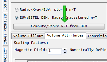
8. If you forgot (or missed an opportunity) to compute the n-T distribution and/or the rendering grid, compute them by pushing the ‘Models → Volume Attributes → Compute/Store N-T from DEM’ (blue arrow) and ‘Volume View → Compute Rendering Grid’ (green arrow) buttons, respectively.
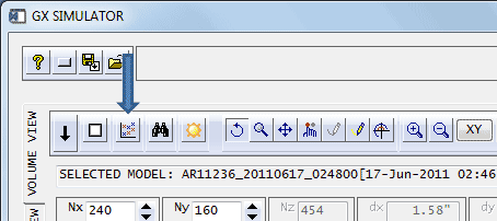
9. In the panel ‘Scanner’, choose the required rendering routine (blue arrow), e.g. ‘...radio_nonflaringsystem_typeMWGR_Transfer_64.pro’ for computing the gyroresonance and free-free microwave emission, or ‘...aiaAIA.pro’ for computing the EUV emission. Then push ‘Compute Radiation Maps’ (green arrow) to start computation.
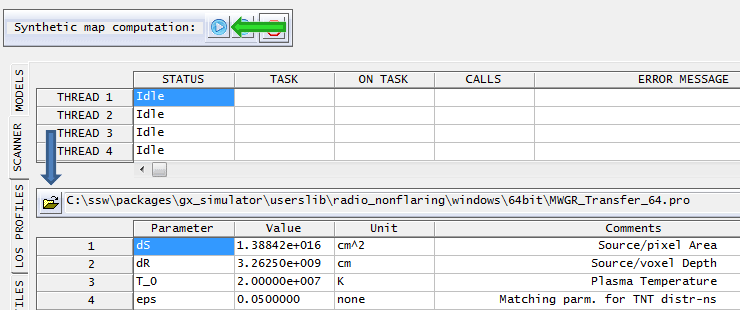
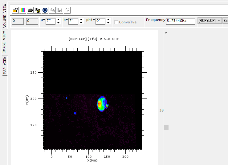
10. In the panel ‘Image View’, track the progress of computation and inspect the emission maps.
11. Use other GX functionality to inspect and modify the model and compute emissions.