How to use 3D models of AR 11809 (2013-08-03)

1. This is a ‘generic’ model, which means that it is defined on a regular grid; no chromospheric model has been added. In addition, no reference FOV map has been added, so the data cube is placed at the center of solar disk (not at the AR actual location). The magnetic data cube is produced by Wiegelmann code with photospheric preprocessing applied. This model is not intended for the data-to-model comparison, but to synthesize various emissions only.

2. This model will let you to reproduce the results presented at AGU 2015 Fall meeting, Radio Emissions from Plasma with Electron Kappa-Distributions. Please, cite this abstract while using these models, and a paper Kuznetsov et al. (2017, in preparation).

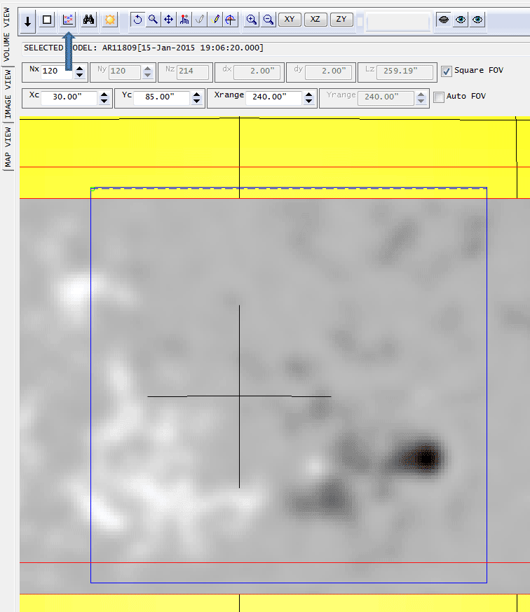
3. To reproduce the results presented in the videos, use the following FOV (Xc, Yc, Xrange) and the following image resolution (Nx). Do not forget to compute the rendering grid.

4. To reproduce the sequence of convolved maps in radio, use a=b=50’’ for radio and a=b=1.2 for EUV in the tab ‘Image view.’

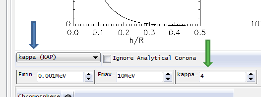
5. To obtain the corresponding radio maps for the case of kappa distribution, do the following (i) import MWGR_Transfer_Slice_64.pro rendering routine at the ‘Scanner’ tab; (ii) select ‘kappa’ from the drop-down menu at the ‘Model/volume fill out’ tab; and (iii) select value of the kappa index in the corresponding window

6. Compute emission at a frequency range of your choice.