How to use 3D models of AR 12158 (2014-09-10)
1. Needed soft: IDL (8.0 or above)/SSW + GX_Simulator (preinstalled from SSW/packages: Solar software http://www.lmsal.com/solarsoft/).
2. Save all provided files in a local folder. This collection of files will let you to reproduce the results presented in Solar ALMA: Observation-Based Simulations of the mm and sub-mm Emissions from Active Regions.
3. Launch GX_Simulator: IDL> GX
4. In the tab "Volume View" upload one of two available models (the only difference between these two models is that in _SteadyHeating model the pairs of (n, T) in each coronal voxel are computed based on an analytical steady state heating model, while in the _EBTEL model these pairs are computed as moments of the EBTEL-provided DEMs) using
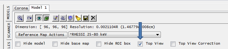
5. In the "Models" tab select "Top view" —needed because the model has a variable z step, which currently cannot be handled by GX Simulator other than from the top view. The direction of the magnetic field vector can be restored to the original one in each voxel by check marking ‘Top view correction’
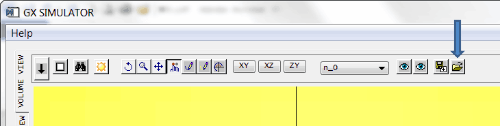
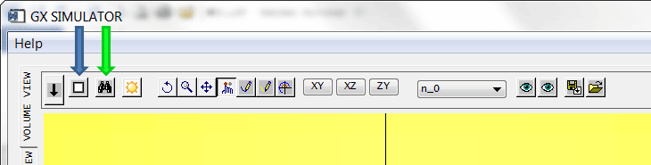
6. In the tab "Volume View" push button "Compute inscribing FOV" (blue arrow) and, once complete, "Zoom to FOV" (green arrow)
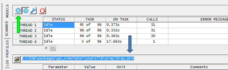
7. To compute EUV emission in SDO/AIA filters, make sure that "C:\SSW\packages\gx_simulator\userslib\euv\AIA.pro" is selected in the "Scanner" tab and hit the button "Scan FOV". Make sure that the desired way of EUV computation is selected in the "Models" tab, e.g., EUV: DEM with TR contribution.
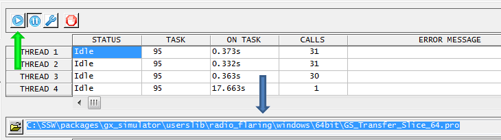
8. To compute MW (GS+FF) emission, select non-LTE fast code, e.g., "C:SSWpackagesgx_simulatoruserslibradio_nonflaringwindows64bitAR_GRFF_nonLTE_64.pro", in the "Scanner" tab and hit the button "Scan FOV".
9. Use the GX functionality to inspect and modify the model and compute emissions.